CFD · Numerical methods · C++ · Summer 2026
NACA 0012 CFD: From Commercial CFD to a C++ Solver From First Principles
The same aerofoil solved twice. First in ANSYS Fluent and validated against NASA measurements, then with a solver written from scratch in C++, because the first study kept raising the question of what the commercial code was doing between the mesh and the answer.
- C++17
- Python
- NumPy
- Matplotlib
- ANSYS Fluent
- 3.6 %
- Lift against NASA SST
- 539 → 5
- Peak cell aspect ratio
- 2.3×10⁻⁷
- Lift at zero incidence
- y⁺ ≈ 1
- Resolved to the wall
Cl = 1.119 against a three-code NASA mean of 1.079 at 10° and Re = 6×10⁶
The first O-grid was measured, diagnosed and rebuilt rather than used
Symmetry check on the turbulent solution, where the exact answer is zero
Mean y⁺ of 1.07 in the converged solution, with no wall functions anywhere
01 Overview
The same aerofoil, solved twice
One aerofoil, a NACA 0012 at 10° incidence and a chord Reynolds number of 6×10⁶, and two goes at it. The first was in ANSYS Fluent, validated against NASA surface-pressure data, and it answered whether the result could be trusted. The second was a solver written from scratch, and it exists because the first study kept raising a question it had no way of answering: what was happening between the mesh and the answer.
That precursor is the short section immediately below. The rest of the page is the solver. It implements the numerical machinery a commercial code keeps out of sight: the finite-volume discretisation, the pressure-velocity coupling that makes incompressible flow solvable at all, the correction that keeps a skewed mesh honest, and a two-equation turbulence model with its near-wall treatment. There is no numerical library underneath it. The linear systems are solved by a Gauss-Seidel sweep with over-relaxation written for this project, and no discretisation, no boundary condition and no turbulence closure comes from a library.
The discipline that makes it worth showing is not that it runs. It is that every stage was checked against a problem whose answer was already known, before being trusted on a problem whose answer was not. At the end the two solutions meet: the same section, the same incidence, the same Reynolds number, one answer from a commercial code and one from a few thousand lines of C++.
Aerofoil geometry
200 surface nodesNACA 0012 thickness distribution evaluated analytically, cosine-spaced, closed trailing edge
Structured O-grid
Quality metricsAlgebraic generator with surface-normal launch, Bezier radial lines and Laplacian smoothing
Diffusion operator
p → 2Laplace solver verified against an analytical annulus solution for observed order of accuracy
Convection schemes
p → 2 and 1Central differencing and first-order upwind measured against a one-dimensional analytical solution
SIMPLE coupling
Ghia et al.Built on a staggered lid-driven cavity and validated against the Ghia benchmark before going near an aerofoil
Collocated solver
Re = 100Operators generalised to the body-fitted grid with Rhie-Chow interpolation and non-orthogonal correction
k-omega SST
Re = 6×10⁶Two-equation RANS closure on a wall-resolved mesh designed for y⁺ ≈ 1
Second-order convection
Cl and CdLimited linear-upwind reconstruction applied as a deferred correction, then compared against NASA reference solutions
02 Precursor
The study this came from
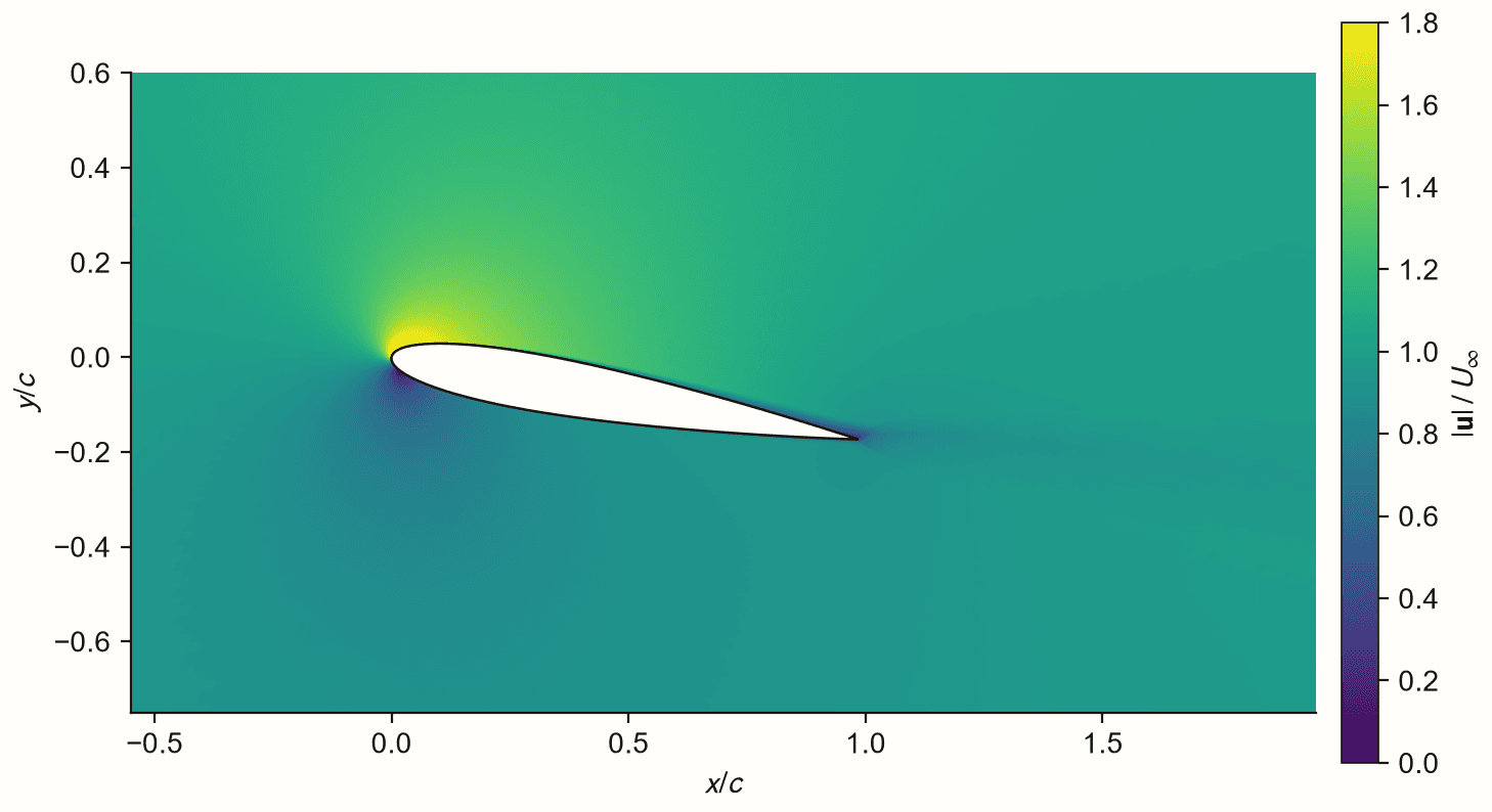
Before any of the code below existed, this aerofoil was solved in ANSYS 2026 R1: two-dimensional steady RANS, 10° incidence, chord Reynolds number 6×10⁶, on a mesh of roughly 27,000 cells with ten inflation layers and a sphere of influence around the section. The case was chosen because high-quality NASA experimental data exists for it, so the argument could be carried to the end instead of stopping at plausibility.
It worked. The computed surface pressure distribution overlaps the NASA data across the full chord, and the integrated lift came out at CL ≈ 1.06 against a measured 1.07 to 1.08, about 1.4 % low, having been predicted at 1.097 by a thin-aerofoil hand calculation done before the solver was opened. Matching the whole Cp distribution is the stronger claim: an integrated coefficient can agree through two errors cancelling, a point-by-point match across the chord cannot.
Velocity magnitude
Static pressure
Validation was against the NASA NACA 0012 resources at matched Reynolds number and incidence: Gregory and O’Reilly for surface pressure, Ladson for force coefficients.
Verification came first and separately. Mass imbalance settled at order 10⁻⁷ of the incoming flow, residuals reached about 10⁻⁶ with flat force monitors rather than residuals alone, and grid and domain independence were set out as a controlled six-case matrix using Richardson extrapolation and the grid convergence index.
That matrix is a plan rather than a result. It was specified and not completed, so the numerical uncertainty on the lift coefficient was never quantified, and the write-up said so.
The rest of the ANSYS study
So the study answered its own question: the result is trustworthy for lift and not for drag, and it can say which is which. What it could not answer is what happened between the mesh and the answer. Choosing a second-order scheme, a coupled solver or a y⁺ target was still selecting from a menu. Everything below is what came of writing the thing each of those options switches on.
03 Numerical method
What the solver actually does
The solver is cell-centred and collocated: velocity components and pressure all live at cell centres. Every transport equation is integrated over a control volume and converted by the divergence theorem into a sum of fluxes through faces, so the discrete equations conserve mass and momentum by construction rather than by accident.
Σf (ρ uf · Sf) φf − Σf Γf (∇φ)f · Sf = Σf Sφ VP
Sf = Ef + Tf
μt = ρ a1 k / max(a1 ω, S F2)
- Why pressure needs its own equation
- In incompressible flow there is no equation for pressure: it appears in the momentum equations but never in continuity. SIMPLE resolves this by predicting a velocity field from a guessed pressure, deriving a pressure correction that forces the face fluxes to conserve mass, then correcting both. The solver iterates that loop with under-relaxation until continuity holds to a set tolerance.
- Why Rhie-Chow is unavoidable here
- Storing velocity and pressure at the same location decouples them on a collocated grid: a checkerboard pressure field produces no force and the solver has no way to reject it. Rhie-Chow interpolation builds the face velocity from a momentum-weighted average that reintroduces the pressure difference between adjacent cells, which suppresses the mode.
- Wall treatment
- The turbulent cases resolve the boundary layer rather than modelling it. Turbulent kinetic energy is set to zero at the wall and the specific dissipation rate is imposed from the near-wall asymptote ω = 60ν / (β₁ y²). This requires the first cell centre to sit at y⁺ of order one, which is what the high-Reynolds-number mesh was designed to deliver.
- Convection, both ways
- The turbulent case is solved twice. First with first-order upwind, which is unconditionally bounded and robust but strongly diffusive. Then with a limited linear-upwind reconstruction added as a deferred correction, keeping the robust operator in the matrix and moving the higher-order contribution to the source term, ramped in gradually.
04 Grid generation
The mesh that had to be rebuilt
The aerofoil is generated analytically from the NACA 0012 thickness equation with the closed-trailing-edge coefficient, distributed with cosine spacing so that points cluster where the curvature is: the leading edge and the trailing edge.
The first O-grid ran. It produced a converged Laplace solution and had no inverted cells, which is exactly the situation in which a mesh gets used without further thought. Because the generator also computed quality metrics, it was measured instead, and the measurement was bad enough to send the generator back for a rewrite.
First attempt
After the redesign
- Peak aspect ratio
- 539.3 → 5.0
- Peak non-orthogonality
- 81.7° → 29.7°
- Face-vector closure
- 5.6×10⁻¹⁷
A hundredfold reduction in the worst cell
Below the threshold where explicit correction can cope
Cell faces sum to zero at machine precision
05 Verification
Checking the operators before trusting them
Verification asks a question that has nothing to do with aerodynamics: given these equations, does the code solve them correctly, and at the rate the discretisation promises? It is answered against problems with closed-form solutions, where any discrepancy is the code's fault rather than the physics model's.
Once the operators were generalised to the body-fitted grid, the geometric machinery was tested on its own terms: face ownership and connectivity, cell areas, the closure of face vectors around every cell, mass conservation under a uniform flow imposed exactly, and the Green-Gauss gradient of a linear pressure field with a known answer.
- Uniform-flow mass residual
- 1.1×10⁻¹⁶
- Linear pressure-gradient error
- 2.3×10⁻¹²
- Invalid or collapsed cells
- 0
31,400 interior faces, 200 wall, 200 far field
Against the exact ∇p = (2, −3)
Every cell closes and carries the expected face count
The same diffusion operator was then run on the aerofoil grid itself, where no analytical solution exists. What can still be checked is conservation: whatever diffuses out of the wall must arrive at the far field.
Integrating the flux over each boundary gives 1.7904 leaving the wall and 1.7904 arriving at the far field, a net imbalance of 8.2×10⁻⁷, or a relative imbalance of 4.6×10⁻⁷. A discretisation that leaked would show up here even though the exact field is unknown.
06 Validation
The cavity before the aerofoil
SIMPLE was not written directly onto the aerofoil grid. It was built first on the lid-driven cavity, a square box with a sliding top, on a staggered Cartesian arrangement where the pressure-velocity coupling is simplest and the failure modes are best understood. The cavity at Re = 100 has been a reference case since Ghia, Ghia and Shin published tabulated centreline velocities in 1982.
Agreement on one grid is weak evidence: a solver can match a benchmark at a single resolution by luck or by compensating errors. What is worth more is the way the error behaves under refinement.
Root-mean-square error against the benchmark falls from 0.0157 to 0.0078 to 0.0033 on the u profile as the grid doubles twice, which is close to first order.
That rate is itself a check. The cavity solver uses first-order upwind convection, and the one-dimensional verification measured that scheme at order 0.95. The validation error is falling at the rate the verification predicted, which ties the two exercises together rather than leaving them as separate claims.
Verification
Am I solving the equations correctly?
- Diffusion operator measured at order 1.9988 against an analytical annulus
- Convection schemes measured at order 2.00 and 0.95 against a one-dimensional exact solution
- Face-vector closure and uniform-flow conservation at machine precision
- Green-Gauss gradient of a linear field correct to 2.3×10⁻¹²
- Boundary flux balance closed to 4.6×10⁻⁷ on the aerofoil grid
Validation
Do the equations describe the real flow?
- Lid-driven cavity centreline velocities against Ghia et al. (1982) on three grids
- Zero lift recovered at zero incidence on a symmetric section, to 2.3×10⁻⁷
- Turbulent lift and drag against three independent NASA reference codes
The numerical operators are verified in the strict sense: measured orders of accuracy, not just converged residuals. Validation is real but partial. The cavity and the symmetry check are solid; the turbulent aerofoil case is compared against reference CFD rather than experiment, on a single grid, and with freestream turbulence settings that do not match the reference. It is a credible solver, not a validated one.
07 Development
A laminar case to develop against
Before turbulence, the collocated solver was exercised on the aerofoil at Re = 100, where the flow is steady and laminar and the equations being solved are unambiguous. This is where Rhie-Chow interpolation and the non-orthogonal correction were shaken out.
An earlier attempt to run the momentum equations on their own, with pressure frozen, is worth recording because of how it failed. Without a pressure correction enforcing continuity there is nothing to stop the velocity field growing without bound, and the run diverged to non-finite values in every one of the 15,800 cells. That is the correct behaviour for an incompressible momentum predictor with no coupling, and it is the most direct demonstration of why SIMPLE exists.
08 Turbulence
Resolving the wall at Re = 6×10⁶
Moving to a chord Reynolds number of six million changes the problem entirely. The boundary layer becomes a thin turbulent sheet, and the solver has to gain a turbulence model and a mesh capable of resolving that sheet without wall functions.
Flow conditions
- Reynolds number
- 6.0×10⁶
- Incidence
- 10°
- Formulation
- Incompressible, non-dimensional
- Turbulence model
- k-omega SST, fully turbulent
Wall-resolved mesh
- Nodes
- 240 × 180
- Cells
- 42,960
- First node spacing
- 9.23×10⁻⁶ c
- Wall-normal growth ratio
- 1.064
A wall-resolved mesh is not produced by refining until it looks fine. The first cell height is computed from an estimate of the wall shear stress, which sets the viscous length scale, which sets the spacing needed to place the first cell centre inside the viscous sublayer.
That calculation gave a first node spacing of 9.23×10⁻⁶ chords, grown outward at a ratio of 1.064. The consequence is cells with edge aspect ratios in the hundreds, which would be a defect on the laminar grid and is the intended design here: the boundary layer varies violently normal to the wall and hardly at all along it, so the cells should be stretched to match.
Before running the case of interest, the turbulent solver was run at zero incidence. A symmetric section at zero angle of attack must produce exactly zero lift, so any lift the solver reports is pure numerical and modelling error, with no physics hiding it. It is the cheapest severe test available for this configuration.
09 Discretisation study
What the convection scheme costs
The turbulent case was solved twice on the same mesh with the same turbulence model, changing only how convected quantities are evaluated at faces. The first-order upwind solution converged to every tolerance and looks entirely reasonable. It is also wrong in a way that only a comparison exposes.
| Quantity | First-order upwind | Limited second-order |
|---|---|---|
| Lift coefficient Cl | 1.0064 | 1.1187 |
| Drag coefficient Cd | 0.04731 | 0.01326 |
| Pressure drag Cd (pressure) | 0.04272 | 0.00733 |
| Viscous drag Cd (viscous) | 0.00459 | 0.00593 |
| Peak turbulent viscosity ratio | 1438 | 747 |
The pressure drag falls by a factor of nearly six. That number is the numerical diffusion of the first-order scheme made visible: smearing gradients across cells thickens the effective boundary layer, weakens the suction peak and leaves a pressure imbalance that is a discretisation artefact rather than aerodynamics.
The peak turbulent viscosity ratio tells the same story from the model's side. The first-order solution carries almost twice the peak eddy viscosity of the second-order one. Numerical diffusion thickened the shear layer, the turbulence model saw the thickened profile and responded by producing more turbulence, and the two errors reinforced each other.
10 Comparison
Against the NASA reference solutions
The NASA Turbulence Modeling Resource publishes this exact case, a NACA 0012 at 10° and Re = 6×10⁶, solved with the SST model by three independent codes on a common 897 × 257 grid. Because the three agree closely with each other, they form a usable reference band.
| Source | Cl | Cd |
|---|---|---|
| This solver, second order | 1.1187 | 0.01326 |
| CFL3D | 1.0778 | 0.01236 |
| FUN3D | 1.0840 | 0.01253 |
| NTS | 1.0765 | 0.01251 |
| Deviation from the three-code mean | +3.6 % | +6.4 % |
11 Limitations
What this solver is not
- Two-dimensional and incompressible. No compressibility, no three-dimensional effects, and no route to either without substantial rework.
- No transition model. The boundary layer is turbulent from the leading edge, which matches the NASA case intent but rules out any case where transition location matters.
- The second-order result is not fully converged. Continuity met its tolerance; the momentum and turbulence increments did not before the iteration cap.
- One grid at Re = 6×10⁶. Grid convergence was demonstrated at Re = 100 and not repeated for the turbulent case, so the discretisation uncertainty on the headline coefficients is unquantified.
- An O-grid, not a C-grid. Production aerofoil meshes use a C-topology precisely because an O-grid under-resolves the wake, which is visible in the turbulent viscosity field.
- Reference conditions do not match. Compressibility, freestream turbulence and grid density all differ from the NASA solutions being compared against.
- A custom implementation, not a production code. It reproduces published behaviour on the cases tested here. That is a long way short of the validation coverage behind any code used for engineering decisions.
12 Reflection
What building it changed
- Convergence is not correctness. The first-order turbulent solution met every tolerance and over-predicted drag by nearly a factor of four. Residuals measure whether iteration has stopped moving, not whether the answer is right.
- Mesh quality is a physics decision. A mesh that runs cleanly can still bias the answer, and the only way to know is to measure it before solving rather than after.
- Discretisation order shows up in drag first. Lift is an integrated pressure difference and forgiving; drag depends on gradients and exposes numerical diffusion immediately.
- Canonical problems earn their keep. The annulus, the one-dimensional profile and the cavity each cost little and each caught something. The measured upwind order later explained the cavity's convergence rate and predicted the turbulent drag error.
- Commercial CFD reads differently now. Choosing a second-order scheme, a coupled solver or a y⁺ target in Fluent is no longer selecting from a menu, because I have written the thing each option switches on.
The complete write-up lives in the repository: methods, data, code, provenance and limitations.
github.com/Jadbadawi/naca-cfd-solver