CFD · FEA · Multiphysics · Summer 2026
Wind Turbine Aero-Structural Simulation
A rotating-frame RANS solution of a three-bladed rotor, coupled one way into an orthotropic composite shell model of the blade, then assessed for what it can and cannot support.
- 0.116 %
- Reaction vs hand calc
- 0.07 %
- Tip speed vs ΩR
- 0.405 m
- Tip deflection
- Not validated
- Rotor performance
Root radial reaction 1,578.1 kN from ANSYS against 1,576.3 kN from mΩ²r
98.05 m/s in CFD-Post against 98.12 m/s by hand
0.92 % of the 44.2 m rotor radius
No matched experimental data; Cp is a coarse-grid value
01 Problem
The engineering problem
A three-bladed horizontal-axis wind turbine sits in a 12 m/s wind and turns at 2.22 rad/s. The question is what aerodynamic load that produces on a blade, and what the blade does under it.
Answering it takes two physics domains. A steady RANS solution in a rotating reference frame predicts the pressure field on the blade surface; that field is then mapped onto a separate structural mesh, where an orthotropic composite shell model predicts deformation, stress and root reactions. The coupling runs one way only: the structure never feeds its deformation back to the flow.
Only one blade is solved. Rotational periodicity across a 120° sector stands in for the other two, on the assumption that all three blades and their inflow are identical. That single assumption cuts the cost of the aerodynamic problem by roughly a factor of three, and it is the first thing this page holds up to scrutiny.
02 Method
The simulation workflow
Operating condition
Inputs12 m/s axial wind, 2.22 rad/s rotor speed, 44.2 m tip radius. Fixes the tip-speed ratio at 8.18 and the local relative wind at every radius.
Rotating-frame RANS
ANSYS FluentSteady incompressible pressure-based solve on a 120° periodic sector, SST k-ω closure, frame motion applied to the fluid cell zone instead of moving the mesh.
Aerodynamic pressure and torque
OutputsSurface pressure on the blade wall, plus the integrated moment about the rotor axis that gives torque and, scaled by three, rotor power.
Pressure mapping
WorkbenchThe pressure field is interpolated from the CFD wall mesh onto a different structural mesh. This step is where a multiphysics workflow can lose load without any warning.
Orthotropic shell FEA
ANSYS MechanicalSHELL181 elements on the blade midsurface, homogenised orthotropic composite, linearly tapering skin and spar, mapped pressure plus centrifugal inertia, remote displacement at the root.
Structural response
OutputsTotal deformation, equivalent stress, root force and root moment reactions.
Verification and credibility assessment
AssessmentIndependent hand calculations, convergence evidence and an explicit statement of what the model has not yet earned the right to claim.
Each stage consumes the previous one's output, so an error anywhere propagates forward silently. A structural stress contour looks exactly the same whether the pressure field feeding it was converged or not.
Aerodynamic model
- Rotor radius
- 44.2 m
- Wind speed
- 12 m/s
- Angular speed
- 2.22 rad/s
- Tip speed ΩR
- 98.12 m/s
- Tip-speed ratio λ
- 8.18
- Flow model
- Steady RANS
- Turbulence closure
- SST k-ω
- Rotor representation
- 120° periodic sector
- Baseline mesh
- 367,691 cells
- Solver
- ANSYS Fluent
Structural model
- Idealisation
- Shell midsurface
- Elements
- 4,831 SHELL181
- Structure
- Outer skin + spar
- Material
- Homogenised orthotropic
- Stiffness ratio E1/E2
- 15
- Skin thickness
- 0.100 m to 0.005 m
- Spar thickness
- 0.100 m to 0.030 m
- Loads
- Mapped pressure + Ω²r
- Root
- Remote displacement
- Solver
- ANSYS Mechanical
03 Physical modelling
Making a spinning rotor a steady problem
A rotor is neither steady nor small. Solved literally, it needs a moving mesh, a transient solution and the full 360° of azimuth. Two modelling decisions remove all three costs, and both are worth stating precisely because both buy their speed with an assumption.
The rotating reference frame. Instead of rotating the mesh, the governing equations are written in a frame that rotates with the rotor. The blade is then stationary relative to its own cell zone, the flow field around it stops changing with time, and a steady solver is legitimate. The price is two extra acceleration terms in the momentum equation.
Ω × (Ω × r)
2 Ω × urel
There is no Euler term, because Ω is constant at a fixed operating point. Fluent introduces both source terms once frame motion is enabled on the fluid cell zone, which means the entire physical difference between a rotating and a stationary analysis lives in a setting that is easy to leave switched off and impossible to see in a contour plot afterwards.
The 120° sector. A three-bladed rotor repeats itself every 360°/3 = 120°, so one sector containing one blade can represent the whole machine if the two radial faces are joined as a rotational periodic pair. Flow variables leaving one face re-enter at the other, rotated by 120°.
360° / 3 = 120°
04 CFD
Aerodynamic loading and rotor power
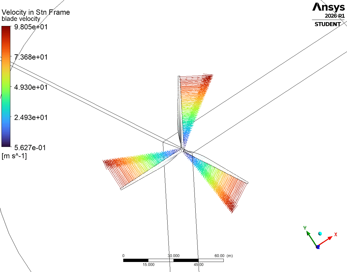
The first result to check is kinematic, because it is the one with an exact answer. Blade velocity in the stationary frame reaches 98.05 m/s at the tip against 98.12 m/s from ΩR by hand, a difference of 0.07 %. That single number verifies the rotation rate, the axis, the units and the 1 m root offset at once. It says nothing whatever about the aerodynamics.
Sectional pressure
Sectional velocity
Torque follows from integrating the surface pressure and shear moment about the rotor axis. The supplied course result gives a one-blade torque of 137,115 N·m, and the rest is arithmetic: three blades at 2.22 rad/s give 0.913 MW of mechanical rotor power, against 6.496 MW of kinetic power passing through the 6,137 m² swept area.
CP = Protor / (½ ρ A V∞3) = 0.913 / 6.496 = 0.141
05 Verification
Numerical credibility
Convergence is not an iteration count. A run that stops at the number of iterations it was asked for has demonstrated nothing except that the loop finished. What matters is whether the residuals are small and the engineering outputs have stopped moving, judged together.
The figure below is the integral static pressure on the blade wall, logged every iteration of my own run of the baseline case. It is the quantity the structural analysis ultimately consumes, so it is the right thing to watch.
Three further numerical questions sit above that one, in the order they need answering:
- Mesh independence. The 367,691-cell baseline resolves the workflow, not the physics. The supplied refinement evidence puts Cp still in motion at multi-million-cell counts, so discretisation error is currently the dominant uncertainty in every aerodynamic number on this page.
- Near-wall resolution. SST k-ω earns its reputation in adverse pressure gradients only if the near-wall mesh matches the treatment it is being asked to use. Wall shear, and therefore y⁺, is an output rather than an input, so the y⁺ distribution has to be plotted after solving and audited against the intended range across the whole blade, not assumed from the first-cell height.
- Domain and boundary sensitivity. The far field is a numerical stand-in for an unbounded flow, and the wake needs room to develop downstream. Inlet turbulence intensity and viscosity ratio are estimates, not measurements, so their influence on torque has to be bounded rather than trusted.
06 Multiphysics
Crossing the interface
pCFD(x) → pFEA(x)
This is what makes the analysis one-way. Pressure crosses from fluid to structure; deformation does not cross back. The aerodynamic solution therefore remains that of the undeformed blade, and the local twist that actually sets angle of attack is never updated. For a first aero-structural estimate at a moderate operating point that is a reasonable trade, and the tip deflection below is what decides whether it holds.
The interpolation itself deserves more suspicion than it usually gets. Mapping between non-matching meshes is a numerical operation with its own error, and a coverage report showing 100 % of target nodes received a value is not evidence that the load survived the trip. Two meshes can both be fully covered and still disagree about the total force.
07 FEA
The structural idealisation
The blade is a slender, twisted, hollow composite shell: an aerodynamic skin over an internal spar, both tapering from root to tip. It is modelled as curved shell surfaces carrying an assigned thickness rather than as a solid meshed through its wall.
- Why shell elements
- The blade is 43.2 m long and a few centimetres thick. Shell theory stores the midsurface and reconstructs the through-thickness strain analytically, so the wall costs one element instead of the several needed to resolve bending through a solid. Resolving 44 m of span with solids at that wall thickness is not a modelling improvement, it is an unaffordable one.
- Tapering thickness
- The skin runs from 0.100 m at the root to 0.005 m at the tip and the spar from 0.100 m to 0.030 m, both linear. Thickness is a property of the shell section rather than geometry that has to be meshed, which is precisely what makes the idealisation cheap.
- Homogenised orthotropy
- One orthotropic material stands for the whole laminate: E₁ = 113.75 GPa along the span against 7.583 GPa across it, with matched shear moduli and Poisson ratios. It captures directional stiffness globally and represents no individual ply, no stacking sequence and no adhesive layer.
- Loads and support
- Mapped aerodynamic pressure plus centrifugal inertia from the 2.22 rad/s rotation, reacted by a remote displacement at the root standing in for the hub connection. Gravity is omitted, and the pressure object carries no aerodynamic wall shear.
08 Verification
The check that carries the most weight
For a rigidly rotating mass distribution, the total radial force reduces exactly to the total mass times the square of the angular speed times the centre-of-mass radius, no matter how the mass is spread along the span. That makes it computable by hand, independently of the finite element model, from three quantities the model reports.
Fc = m Ω2 rcm = 22,473 × 2.222 × 14.232
- Analytical
- 1,576.3 kN
- ANSYS
- 1,578.1 kN
- Difference
- 0.116 %
mΩ²r by hand
Root radial reaction
Well inside any reasonable tolerance
09 Results
Structural response
The blade deflects away from the incoming wind, which is the direction the mapped pressure field demands, and the profile is classic cantilever behaviour: near zero at the root, growing non-linearly outboard, because every span station carries the integrated moment of all the load outboard of it.
Maximum tip deflection is 0.405 m, or 0.92 % of the 44.2 m rotor radius. That number does double duty. On a real machine it is a design driver, because the blade must not strike the tower. Here it is also the test of whether one-way coupling was legitimate in the first place, and under 1 % of radius the assumption looks defensible at this operating point.
The qualification matters: deflection magnitude is not the quantity aerodynamics is most sensitive to. Local twist sets angle of attack, and a small tip displacement accompanied by significant torsional rotation could still change the loading materially. The change in twist was not extracted, so the one-way assumption is supported rather than proven, and under a peak gust the conclusion could reverse.
The supplied structural results give a maximum equivalent (von Mises) stress of approximately 33.36 MPa, at the junction where the spar transfers bending load into the skin. That location is physically sensible, and it is also exactly the sort of place where a value is sensitive to CAD simplification, to how the spar and skin are connected, and to local mesh density.
Against the 537 MPa tensile strength quoted for the material, the ratio is about 16.
10 Judgement
Modelling decisions
Every choice below buys something and costs something. Listing the cost beside the benefit is what separates a model from a set of settings.
| Decision | Why | What it costs |
|---|---|---|
| Steady RANS | Affordable prediction of mean rotor loading | No transient or unsteady effects |
| SST k-ω | Good near-wall behaviour in adverse pressure gradients | Depends on a matching near-wall mesh |
| Rotating reference frame | Steady solution without a moving mesh | Fixed operating point only |
| 120° periodic sector | One third of the cells | Requires exact threefold symmetry |
| Shell FEA | Efficient for a slender composite blade | No detailed 3D local stress state |
| One-way FSI | Cheap first aero-structural estimate | Deformation never alters the flow |
| Homogenised orthotropy | Captures directional stiffness globally | No ply-level behaviour or interface |
11 Scope
What the model does not yet prove
Verification
Did I solve the chosen model correctly?
- Tip speed against ΩR: 98.05 vs 98.12 m/s, 0.07 %
- Root radial reaction against mΩ²r: 0.116 %
- Cp below the Betz limit of 0.5926
- Load-path direction: radial force in x, bending moment in y
- Still outstanding: mesh convergence, y⁺ audit, load-transfer conservation
Validation
Does the model represent reality closely enough?
- Requires measured rotor torque and thrust at matched V∞, Ω and pitch
- Requires blade surface pressure or sectional force distributions
- Requires measured deflection or strain under the same load
- Requires wake velocity deficit and swirl at defined planes
- Requires the measurement uncertainty to compare against
No matched experimental dataset was available for this turbine, so the model must not be described as experimentally validated. Everything on this page is verification, plausibility assessment or engineering judgement. Those are different claims, and conflating them is how an unvalidated model ends up carrying a design decision.
More specifically, and in no particular order of severity:
- CFD mesh independence is not demonstrated. The supplied refinement evidence shows Cp still moving well beyond the baseline mesh.
- Iteration independence is not demonstrated. The blade pressure monitor was still drifting 0.41 % across the final 100 iterations of the baseline run.
- Structural mesh convergence has not been established. The 4,831-element mesh has not been refined and compared.
- Force and moment conservation across the pressure transfer has not been quantified.
- The homogenised orthotropic material represents no individual ply, no stacking sequence, no adhesive layer and no spar-to-skin bondline.
- One-way coupling ignores aerodynamic feedback from deformation, and the change in local twist was never extracted.
- The steady periodic model excludes asymmetric and transient effects: tower shadow, shear, yaw, gusts and blade-to-blade variation.
- Gravity was omitted, so the once-per-revolution gravitational load that matters for fatigue is absent.
- Composite failure needs a directional criterion, not von Mises against a tensile strength.
- Run under the ANSYS Student licence, which caps mesh size and therefore limits how far the refinement study can be taken on this machine.
12 Future work
The next verification campaign
None of the following has been run. It is the ordered plan for turning the current model into one whose numbers could carry an engineering argument, with the largest source of uncertainty attacked first.
- 01
CFD mesh convergence
Three systematically refined meshes at a constant refinement ratio, tracking Cp, torque, thrust and y⁺ statistics, with Richardson extrapolation and a grid convergence index once the sequence is in the asymptotic range.
- 02
Load-transfer verification
Compare the resultant force and moment reported by Fluent against the same resultants integrated over the mapped structural load, and report the percentage difference rather than the node coverage.
- 03
Structural mesh convergence
Refine the shell mesh and track tip displacement, root force, root moment, total strain energy and a representative stress away from geometric singularities.
- 04
Load separation
Solve aerodynamic pressure alone, centrifugal loading alone, then combined, so each contribution to deflection and stress can be attributed rather than inferred.
- 05
Parameter sweep
Automate the operating point across wind speed and rotor speed to trace Cp against tip-speed ratio, and the structural response along with it, instead of characterising one machine by one point.
- 06
Sensitivity assessment
Bound the influence of the modelling inputs that were estimated rather than measured: inlet turbulence quantities, orthotropic stiffness constants and the root support idealisation.
The complete write-up lives in the repository: methods, data, code, provenance and limitations.
github.com/Jadbadawi/aerospace-cfd-fsi