CFD · Verification & validation · Summer 2026
NACA 0012 Aerofoil: Verification and Validation
Carrying a two-dimensional RANS solution from a hand calculation through to a point-by-point comparison against NASA measurements, and reporting the part of the mesh that does not support the answer.
- 1.4 %
- Lift vs experiment
- 1.097
- Thin-aerofoil prediction
- 10⁻⁷
- Mass imbalance
- y⁺ audit
- Failed, and reported
CL ≈ 1.06 against NASA measurements of 1.07 to 1.08
Computed before the solver was opened, so the CFD was falsifiable
Normalised against the incoming flow
Much of the surface sits outside the range the wall treatment needs
01 Overview
Why this case
A CFD result only means something if you can show why it should be believed. This study is a two-dimensional steady RANS solution over a NACA 0012 aerofoil at 10° incidence and a chord Reynolds number of 6×10⁶, run in ANSYS 2026 R1 alongside CornellX's ENGR2000X simulation course on edX.
The case was chosen for one reason: high-quality NASA experimental data exists for it, so the full verification and validation argument can be carried all the way to the end rather than stopping at plausibility. It is the only case in this portfolio where that is true, which is exactly why the wind turbine study, built on the same solver and the same discipline, cannot be called validated.
Note the ordering of the last two steps. Verification comes before validation, and it is not optional: comparing an unverified solution against experiment tells you nothing useful. If it disagrees you cannot tell whether the physics model is wrong or the mesh is too coarse; if it agrees you cannot tell whether it agreed for the right reason.
02 Setup
The physical problem and its domain
The case is steady, turbulent, two-dimensional flow around a symmetric NACA 0012 section at 10° angle of attack, with a 1 m chord and air approaching at 51.45 m/s.
The domain is the region between the aerofoil surface and an outer far-field boundary placed roughly 12.5 chord lengths away. That outer boundary is a numerical stand-in for infinity. The real flow extends indefinitely, so truncating it is an approximation whose adequacy has to be demonstrated rather than assumed.
Before any solver was opened, a thin-aerofoil hand calculation put lift at CL = 1.097. That number is what makes the CFD result falsifiable. Without an independent expectation, any output has to be accepted on faith.
03 Discretisation
Designing the mesh
Mesh design is not a matter of making cells small everywhere, which is both unaffordable and unnecessary. It is a matter of spending cells where the gradients are: the leading edge, the boundary layer, the trailing edge and the wake. The mesh here contains roughly 27,000 cells.
- Boundary layer refinement
- Ten inflation layers were applied around the aerofoil with a growth rate of 1.2. They provide additional resolution normal to the wall, where the strongest velocity gradients occur.
- Local aerofoil refinement
- A sphere of influence with a radius of approximately three chord lengths was used around the aerofoil. Within that region the local element size is approximately 0.05c.
- Wake refinement
- Additional refinement was applied downstream of the trailing edge, to resolve the wake and the downstream velocity gradients it carries.
- Edge biasing
- Bidirectional edge biasing concentrates smaller elements near the leading and trailing edges, where the geometry and the aerodynamic gradients require greater resolution.
04 Post-processing
Aerodynamic results
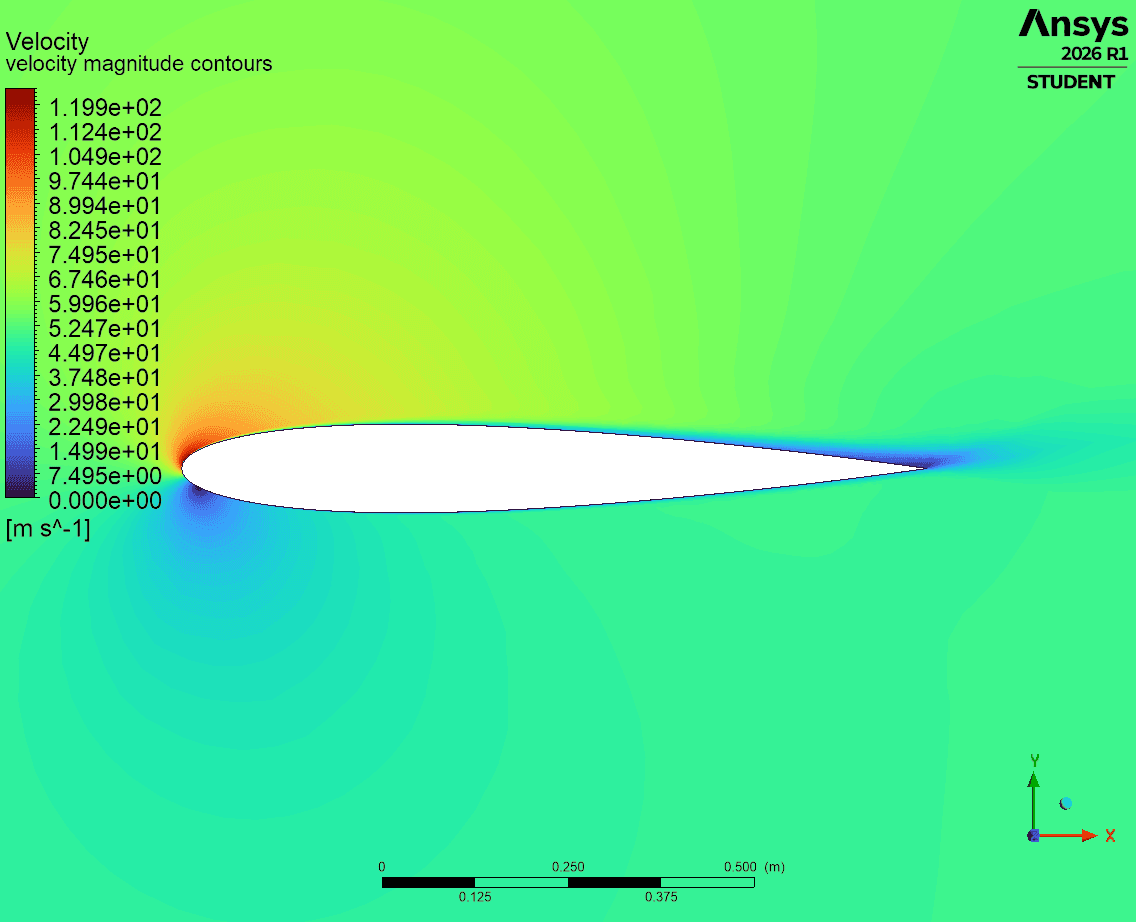
Each field below is checked against what the pre-analysis predicted, rather than just described.
Static pressure
Velocity vectors
The turbulence field is the most diagnostically useful of the four plots, and the one most often skipped. It isolates the boundary layer as a thin high-k sheet, thickening toward the trailing edge and shedding into the wake, which is a direct picture of where turbulent momentum transport is happening.
It also works as a visual mesh check. Turbulence production peaks where mean shear is greatest, very close to the wall. If the near-wall mesh is adequate, that appears as a sharp, well-defined sheet. If it is too coarse, the peak smears across cells and the sheet looks diffuse, a visual symptom of the same resolution problem the y⁺ audit quantifies.
05 V&V
Verification and validation
- Mass conservation. Normalised imbalance of order 10⁻⁷ of the incoming flow.
- Iterative convergence. Residuals driven to ≈10⁻⁶, with flat force monitors rather than residuals alone.
- Near-wall audit. The computed y⁺ distribution checked against the range the chosen wall treatment actually requires, rather than assumed.
- Domain and grid independence. Set out as a controlled six-case verification matrix, one variable changed at a time, each case with a stated acceptance criterion, using Richardson extrapolation and the grid convergence index.
Validation compares the predicted surface pressure distribution against the NASA NACA 0012 resources (Gregory & O'Reilly for surface pressure, Ladson for force coefficients) at matched Reynolds number and incidence. The computed Cp distribution overlaps this experimental data closely across the full chord.
The integrated lift follows at CL ≈ 1.06 against an experimental 1.07 to 1.08, about 1.4 % low, and against the thin-aerofoil hand calculation of 1.097 made before any solver was opened.
Matching the full Cp distribution is a stronger claim than matching lift alone. An integrated coefficient can agree through cancellation between two compensating errors, whereas a point-by-point match across the chord cannot happen by accident. The Cp distribution is also the aerodynamic loading itself, so it is the quantity the structural side of a coupled analysis consumes.
06 Engineering judgement
Where the agreement does not extend
Close agreement on lift is not a licence to trust every output. The mesh supports the pressure field well and the wall shear badly, and those two facts have to be reported together:
- Wall treatment inconsistent with the mesh. Standard wall functions are being applied across a y⁺ field much of which lies outside their valid range.
- Wall-shear-dependent quantities are not supported. Drag is the obvious casualty: the same near-wall limitation that leaves lift accurate leaves skin friction unreliable.
- Grid and domain independence are set out but not completed. The six-case matrix is a plan, not a result, so the numerical uncertainty on CL has not been quantified.
- Trailing-edge cell quality is poor in orthogonality and aspect ratio, in exactly the region that sets the Kutta condition.
- Two-dimensional and fully turbulent throughout. No transition modelling, no three-dimensional effects, no separation onset prediction worth relying on near stall.
The complete write-up lives in the repository: methods, data, code, provenance and limitations.
github.com/Jadbadawi/aerospace-cfd-fsi