CFD · Aerodynamics · 2024/25 · HyPower Bristol, EuRoC 2025
Rocket Airbrake and Fin Aerodynamics
Building a drag model for a rocket's airbrake system, and choosing the fin geometry that had to work with it.
- Star-CCM+
- Autodesk Inventor
- MATLAB
- Abaqus
- OpenRocket
Aerodynamics & Structures Engineer, HyPower Bristol. Waxwing is a team vehicle. This page covers only the aerodynamics work I was responsible for: the airbrake CFD, the airbrake geometry selection, and the fin section and planform selection. Propulsion, avionics, recovery and primary structure were other people's work.
- 25
- CFD cases
- 1.7×
- Drag at full deployment
- 0.041 m
- Boundary layer in CFD
- 0.0661
- Selected fin Cd
Five deployment angles across five freestream velocities
Cd 0.270 deployed against 0.162 stowed, both at 100 m/s
Against 0.047 m from a Prandtl-Schlichting hand calculation
Hybrid section at 10 % thickness, against 0.0670 for the NACA equivalent
01 Overview
The vehicle and the problem
Project Waxwing is HyPower Bristol's entry into the 3 km Liquid category at the European Rocketry Challenge 2025, built out of BristolSEDS at the University of Bristol. It is a student researched and developed bi-propellant vehicle carrying a deployable airbrake system used to trim apogee.
My part was the external aerodynamics. Two things needed answering. The airbrakes needed a drag model before their controller could be tuned, because a controller that modulates drag has to know how much drag it is commanding. And the fins needed a section and a planform chosen on evidence rather than preference. Both problems sit across the subsonic and transonic range, since the vehicle reaches Mach 0.9 early in the burn.
- 01
Trajectory sets the envelope
Simulated trajectories give the Mach, velocity and Reynolds ranges the aerodynamics has to cover, and therefore which cases are worth running.
- 02
Airbrake geometry downselection
Two flap geometries compared on braking force, separation behaviour, and whether their wake would reach the fins.
- 03
CFD sweep
Twenty five steady RANS cases in Star-CCM+, five deployment angles by five velocities, on one meshing setup.
- 04
Verification
Solver output checked against closed form boundary layer theory before any of it was used downstream.
- 05
Drag map delivered
Cd against deployment and velocity, passed to the airbrake control team for gain tuning.
02 Scoping
Why twenty five cases
The vehicle reaches Mach 0.9 about five seconds into flight, with apogee near 3850 m. The airbrakes operate on the coast, at velocities up to 150 m/s.
Compressibility becomes significant above roughly Mach 0.3, which is around 100 m/s at these conditions. The sweep was capped there on purpose, so that the model stayed a clean incompressible one rather than a compressible one with nothing to check it against. The cost of that decision is real and worth stating: the top of the deployment envelope, 100 to 150 m/s, is not covered by these results.
03 Downselection
Choosing the airbrake geometry
Two flap geometries were on the table, a slot design and a rounded petal. The choice was not simply which one produced more drag. A brake that sheds a large separated wake risks that wake reaching the fins, which would put stability at risk at exactly the moment the vehicle is being slowed.
Slot
Petal
The rounded petal produced greater braking force but separated further from the body. The slot design gave less drag with a more predictable separation for a constant base length. The configuration taken forward was a compromise between the two rather than either one outright.
A second constraint came out of the geometry rather than the flow. The number of flaps had to match the number of fins, so the two sit clocked apart and the wake from a brake does not run straight into a fin downstream.
04 Setup
The simulation
- Full geometry, no symmetry plane
- The petals sit clocked out of phase with the fins, so a deployed vehicle is not symmetric about any plane. A half model would have been cheaper and wrong.
- Domain
- A cuboid 24 m by 12 m by 12 m, which is 72.7 by 36.4 by 36.4 rocket radii, with the base of the vehicle 48.5 radii upstream of the outlet.
- Mesh
- Trimmed cell hex dominant core, prism layer mesher at the wall, surface remesher on the body. Base size 4.0 m, 16 prism layers at a stretching factor of 1.5.
- Prism thickness from theory
- Prandtl-Schlichting predicts a 47.2 mm boundary layer at the aft end at 100 m/s, so the prism stack was sized to contain the whole layer rather than guessed at.
- Turbulence model
- Realizable two layer k-epsilon, chosen for cost across twenty five runs and because its all y+ wall treatment adapts to whatever y+ the mesh delivers, so one meshing setup serves every case.
- Wake resolution
- The wake is deliberately coarse. It damps pressure perturbations reflecting off the outlet back onto the body, and for a streamlined shape skin friction dominates, so near wall resolution matters more than wake resolution.
Each case ran to 1000 iterations on a segregated solver, by which point continuity, energy and momentum residuals had fallen to between 10⁻⁷ and 10⁻¹⁰.
05 Verification
Checking the solution before using it
A drag number is only worth handing to a control team if there is some independent reason to believe it. Three checks were run on the solution before any of it was used.
- Local Reynolds number along the body reaches order 10⁷, and the flow turns turbulent within the first 75 mm. That is what justifies a fully turbulent k-epsilon model, rather than the model being assumed to apply.
- Boundary layer height in the solution came out at 0.0408 m against 0.047 m predicted by hand, about 13 percent apart, which confirms the prism stack was tall enough to contain the layer it was sized for.
- Wall y+ was mapped along the body. At 80 m/s fully deployed it sits around 10 across most of the surface, with higher values local to the brakes and fins.
06 Results
The drag map
| Deployment | 20 m/s | 40 m/s | 60 m/s | 80 m/s | 100 m/s |
|---|---|---|---|---|---|
| 0 % | 0.008 | 0.031 | 0.065 | 0.110 | 0.162 |
| 25 % | 0.009 | 0.032 | 0.067 | 0.114 | 0.169 |
| 50 % | 0.010 | 0.035 | 0.076 | 0.130 | 0.193 |
| 75 % | 0.011 | 0.041 | 0.088 | 0.151 | 0.227 |
| 100 % | 0.013 | 0.048 | 0.104 | 0.178 | 0.270 |
Drag rises with both deployment and velocity, and the sensitivity to deployment grows with speed. At 20 m/s the entire deployment range moves Cd by under 0.005. At 100 m/s the same range moves it by more than 0.1. That spread is the reason a single drag figure would not have been sufficient for the controller.
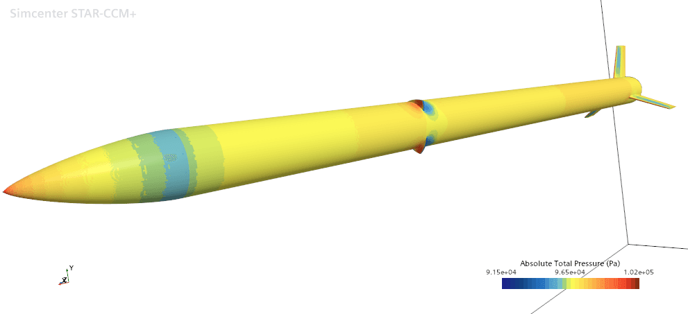
At the petal
Downstream at the fins
Those recirculation regions close quickly, and the flow is reattached by the time it reaches the fins. At this condition the brakes do not compromise fin effectiveness, which was the clearance the mechanical design needed before the geometry could be frozen.
07 Design
Fin section and planform
The fins see both subsonic and transonic flow, since the vehicle passes Mach 0.9 on the way up. A section that behaves well in one regime is not automatically right for the other.
The section tested was a hybrid: a NACA leading edge to keep the flow attached subsonically and delay shock induced separation transonically, then a sharp wedge trailing edge to fix the rear stagnation point and cut wave drag. It was compared against standard NACA sections at three thicknesses, evaluated at the trajectory average condition rather than at a single design point.
| Thickness | Hybrid Cd | Standard NACA Cd |
|---|---|---|
| 10 % | 0.0661 | 0.0670 |
| 12 % | 0.0687 | 0.0691 |
| 14 % | 0.0703 | 0.0715 |
The hybrid at 10 percent thickness gave the lowest drag and was selected. The margin over the equivalent standard section is about 1.3 percent, which is small, and it is worth reporting as small rather than dressing it up. The CFD drag figures were cross checked against a MATLAB panel method written to run over the same geometries, so the ranking rests on two independent methods rather than one.
The planform was chosen separately, through a weighted decision matrix over five candidates. The weightings came from a pairwise comparison of the requirements rather than being assigned directly, and structural stiffness at maximum dynamic pressure, static stability and flutter margin carried three quarters of the weight between them.
| Planform | Weighted score |
|---|---|
| Swept trapezoidal | 3.7 |
| Low aspect ratio swept trapezoid | 3.4 |
| Biconvex cross section upgrade | 3.4 |
| Highly swept clipped delta | 3.3 |
| Elliptical | 2.6 |
Swept trapezoidal won. The elliptical planform lost on manufacturability in composite rather than on aerodynamics, which is worth saying plainly, because a downselection is more useful when the losing reason is specific. Three fins were used rather than four, so the airbrake wake has fewer chances to meet a fin downstream.
The chosen fin was built from three triaxial carbon plies in a [-45, 0, 45] layup. For the structural check I took the worst case flight condition, Mach 0.9 at 850 m with a conservative 15 degree angle of attack, and reduced it to an equivalent uniform pressure of 146 kPa through dynamic pressure and a finite wing lift curve slope, which is what was applied to the Abaqus model of the fin.
08 Limitations
What this does not tell you
These are the assumptions recorded at the time, not ones reconstructed afterwards.
- Panel gaps and manufacturing discontinuities on the body were not modelled.
- The gap between each petal and its housing was not modelled.
- Tri tangent fin tips could not be produced in the CAD package, so they are absent from the geometry. Drag is therefore marginally over predicted at the tips.
- The exhaust hole at the base was left out, to avoid introducing internal flow into a model that had nothing to check it against.
- All surfaces were treated as smooth, including the 3D printed fin tips, which are rougher than the carbon body.
- The sweep stops at 100 m/s, so deployment between 100 and 150 m/s is not covered.